Tutorials

This page shows how to implements the code in various ways.

Random Path Simulator

This example show how to use the basic class Bicycle.

Its initialize a model with one meter between the wheels and max steer angle of 50º. The sim_RandomPath method simulate the model running at a constant speed and a random steer angle for a number of steps, in the example 1m per step for 1000 steps.

import bicycle                          #import the model
import matplotlib.pyplot as plt         #import matplotlib

robot = bicycle.Bicycle(1,50)           #create a robot
robot.sim_RandomPath(1,1000)            #run in a random path

robot.show()                            #show the paths
plt.show()                              #hold the plot

This code will result in a random trajectory of the model plot as a map-like image, its a simple way to get lots of studies cases. The image below show a example of plot from the code, you should get a different result as the code uses a random function.

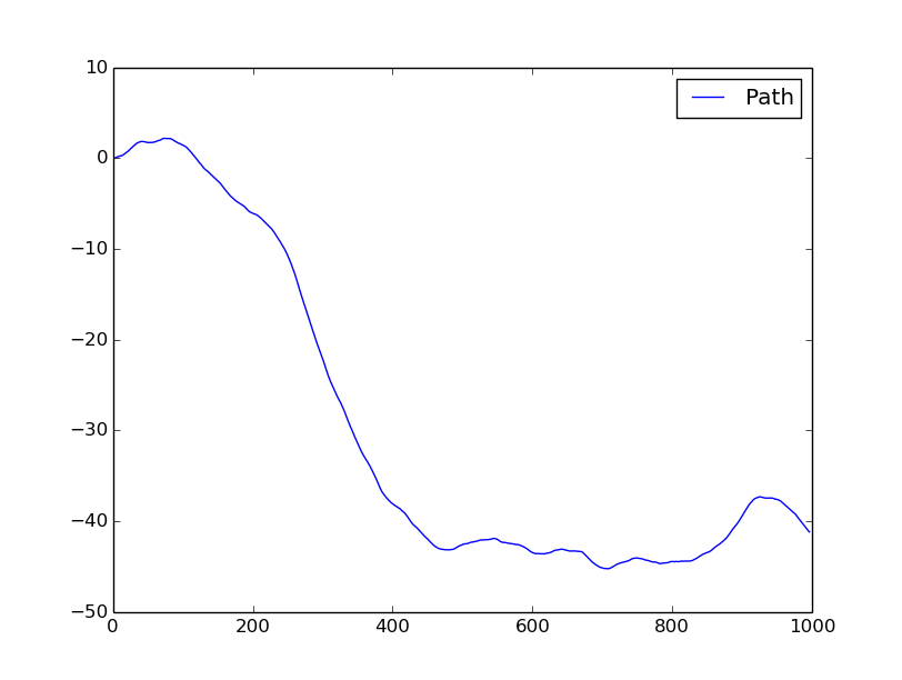
Random path

Odometry Simulator

The vehicle class inherits the features of the bicycle and add some sensors, making possible keep a history of the speeds and the steer angles of the model all through its path.

Real encoders is not perfect(it really away from it in fact), so the simulator add a Gaussian noise to its reads, making it more close to the real world robots , you should set the standard deviation of the noise. The steer angle is assume as a truth information, so no noise is add to it.

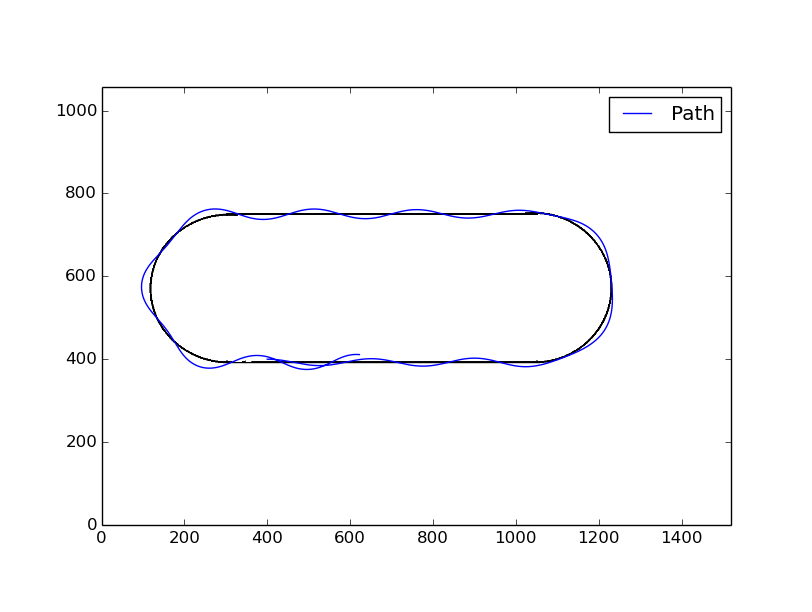
This example create a rectangular path and run it on a vehicle with a noisy encoder, then show the path using directly the sensors data, with no filter, as expected this result in a different path by the propagation of the error in the measurements.

import vehicle                          #import the vehicle model
import matplotlib.pyplot as plt         #import matplotlib

car = vehicle.Vehicle(1,50)             #create a robot
car.setOdometry(True)                   #set the odometer on
car.setOdometryVariance(0.4)            #configure its deviantion to 0.4
speed,angle = [],[]                     #initialize the lists

for a in xrange(4):                     #create a retangular path
    for i in xrange(400):
      angle.append(0)
    for i in xrange(107):
      angle.append(40)
for i in xrange(len(angle)):            #set the speed to a constant along the path
  speed.append(1)

car.sim_Path(speed,angle)               #run in a rectangular path
speed , angle =  car.readOdometry()     #reads the sensors
car2 = vehicle.Vehicle()                #create a second model
car2.sim_Path(speed,angle)              #run it in the path read by odometry

#show the paths
robot.show("Real")
car2.show("Odometry")
plt.show()

Real path and odometry based path

PID Control Simulator

This example implement all the simulator’s features, its use the robot class its load a image file thats represents the “road map” image and run over it autonomously following the black line. The camera class is responsible to sense the environment taking a “slice” of the image and finding the center of the black line on it, if no black line was found at all it return the last error.

The PID controller is a proportional–integral–derivative controller is a control loop feedback mechanism (controller) commonly used in industrial control systems. A PID controller continuously calculates an error value as the difference between a desired setpoint and a measured process variable. The controller attempts to minimize the error over time by adjustment of a control variable, such as the position of a control valve, a damper, or the power supplied to a heating element, to a new value determined by a weighted sum.

A PID controller keep the robot on the path, it apply a steer angle to the model based on the error value get from the camera. The error and the PID result is in a range from -1 to 1 and it is scale to the maximum steer angle.

The robot class need a relation of pixels per meter to scale the map image, in this case its used the default value(375 pxl/meter). The speed of the robot is 5mm or 1.875 pixels per step.

import robot                          #import the model
import matplotlib.pyplot as plt

robot = robot.Robot("Maps/mapao.png") #inicialize the robot in the map
robot.setPose(400,400,0)              #set a initial pose
robot.sim_LineFollower(Steps = 1600,Kp=1,Ki = 0,Kd=0.3,v=0.005,debug=True)

rob.show()  #plot the results
plt.show()  #hold the plot

In this case the debug parameter is True, so the program will print all the errors and the commands from the PID controller. You should get better results, with the robot keeping more closer to the black line, with others gains values in the controller.

Line-Follower robot